Surface water at ocean fronts crosses the winter mixed-layer base within weeks in two submesoscale-resolving models, and the same fields filtered to atlas grid scale resolve much less of it
M. German¹ (co-author slots open) ¹Steps Ventures. Working draft, revision 2, 2026-09-07. Target venue: Biogeosciences (alternative: Ocean Science).
Markers of the form [Pending rerun: ...] flag statements that a running 180-day, moving-mixed-layer, block-bootstrap rerun will replace. They are part of the research record and are removed before submission.
Abstract
Ocean alkalinity enhancement (OAE) removes atmospheric CO2 only while the alkalinity-enriched surface water stays in contact with the atmosphere, and air-sea equilibration takes months. Submesoscale fronts and mixed-layer eddies can move surface water below the mixed layer in days. Global OAE efficiency estimates come from models at roughly 1 degree resolution that do not resolve those scales. We ask how much surface water crosses below the winter mixed-layer base within weeks in two submesoscale-resolving simulations, and how much of that crossing survives when the same velocity fields are spatially filtered to 25 to 100 km. We advect passive particles offline in the 3-D velocity field of MITgcm LLC4320 (about 2 km) in 14 selected subdomains for 16-day winter windows, and in NEMO eNATL60 (about 1.7 km) at the Gulf Stream for 17 days. The diagnostic is a fixed-depth one: a particle counts as crossed if it sits below a 100 m reference depth for at least 80 percent of the last quarter of the window. In nine of the 14 subdomains, 0.16 to 0.38 of the surviving particles cross within the window. In the Baltic, Bass Strait and the Weddell marginal ice zone the fraction is at most 0.001. The same fields filtered to 25 km give 0.00 to 0.08 at 16 days in every subdomain, and in the Antarctic Circumpolar Current series the fraction falls from 0.28 at 2 km to 0.13, 0.045 and 0.00 at 25, 50 and 100 km. The filtered field partially catches up with time: at 25 km it rises from 0.05 to 0.17 between 10 and 22 days while the native fraction stays near 0.25. At the Gulf Stream the two models disagree by a factor of about two (0.16 to 0.20 in LLC4320, 0.39 in eNATL60), and the resolution difference alone cannot produce that gap. The particle bootstrap treats particles as independent, and column clustering alone widens the intervals by at least the square root of three, so the ordering among fronts is not established. Crossing within two to three weeks is fast compared with an air-sea equilibration timescale whose global median we compute as 0.51 yr. The implication for OAE efficiency is a shift of realized uptake beyond the near-term horizon at frontal sites, of a magnitude this study does not quantify. A coupled carbonate calculation and a moving-mixed-layer diagnostic are needed before any efficiency correction is stated.
1. Introduction
Ocean alkalinity enhancement adds alkalinity to seawater. The carbonate equilibrium shifts, the surface ocean holds more dissolved inorganic carbon (DIC) at a given CO2 partial pressure, and atmospheric CO2 is drawn down. The climate benefit is realized only through air-sea gas exchange, which is slow. The equilibration timescale of a surface DIC anomaly is of order months to a year (Jones et al., 2014), and uptake happens only while the alkalinity-enriched water remains in contact with the atmosphere. Any process that moves that water out of the mixed layer before equilibration defers the uptake until the water re-ventilates.
Location-dependent OAE efficiency is now estimated with global ocean models that simulate pulsed alkalinity additions and report the fraction realized as atmospheric uptake over a fixed horizon (Zhou et al., 2024). He and Tyka (2023) studied the near-coast limits of alkalinity addition and the transport that carries it offshore. Tyka (2025) examined how the efficiency metric depends on the horizon and on the treatment of atmospheric pCO2. These models run at roughly 1 degree nominal resolution. They resolve the mean circulation and, in part, the mesoscale, but not the submesoscale (1 to 10 km). Submesoscale fronts and mixed-layer instabilities produce vertical velocities of order 10 to 100 m per day that carry surface water into the interior (Fox-Kemper et al., 2008, Lévy et al., 2012, Omand et al., 2015, Su et al., 2018). Balwada et al. (2018) showed in an idealized channel that a 1 km submesoscale-permitting model subducts about 50 percent more passive tracer than a 20 km model. Whether surface water at realistic open-ocean fronts crosses below the winter mixed layer on timescales shorter than air-sea equilibration, and how much of that crossing is lost when the velocity field is filtered to the grid scale of the efficiency models, has not been reported for a realistic multi-region configuration.
This paper is a model case study, not a global measurement. We advect passive particles offline in two submesoscale-resolving simulations, in 14 selected subdomains of one and one Gulf Stream subdomain of the other, over winter windows of 16 to 22 days. We count the fraction of surviving particles that end the window below a fixed 100 m reference depth and stay there. We repeat the advection in the same velocity fields after spatial filtering to 25, 50 and 100 km. We do not simulate the carbonate system, and we do not compute an OAE efficiency. The paper establishes a transport diagnostic and its resolution dependence within these experiments, compares the crossing timescale with an independently computed equilibration timescale, and states what a coupled calculation would need to add.
2. Data and methods
2.1 Submesoscale simulations
LLC4320. MITgcm LLC4320 at 1/48 degree (about 2 km), 90 vertical levels, hourly output, from the Pre-SWOT regional subsets distributed by NASA PO.DAAC (NASA JPL, 2021, Su et al., 2018). We use 14 regional subdomains (Table 1) in a hemisphere-appropriate deep-winter month: February 2012 for the Northern Hemisphere and July or August 2012 for the Southern Hemisphere. Variables: 3-D u, v, w, potential temperature, salinity, and the KPP boundary-layer depth (KPPhbl), which we use as the mixed-layer-depth proxy. The subdomains were chosen by hand to cover western boundary currents, the Antarctic Circumpolar Current, the Agulhas retroflection, two subpolar deep-convection sites, a subtropical counter-current, tropical and temperate shelves, three enclosed or marginal seas, and a marginal ice zone. They are not an area-weighted sample of the ocean, and every result is for one winter of one year.
eNATL60. NEMO eNATL60 at 1/60 degree (about 1.7 km), with tides, from the SWOT-AdAC interior_daily Zarr archive (Region01, Gulf Stream separation, February to April 2010, daily means, 107 levels) (Brodeau et al., 2020, Uchida et al., 2022). We subset a Gulf Stream front box (35.5 to 40.5 N, 72 to 56 W, matching the LLC4320 WestAtlantic subdomain) over the first 17 days of February 2010 and the upper 350 m. Mixed-layer depth is diagnosed from a 0.03 kg per cubic metre density threshold with a linear equation of state. The two configurations therefore differ in model code, year, tides, mixed-layer definition and output cadence (daily means versus 6-hourly snapshots), in addition to resolution.
2.2 Lagrangian crossing diagnostic
Seeding. Particles are seeded on a regular 0.12 degree grid in the central 50 percent of each subdomain, at 5, 20 and 40 m depth, in every column where the KPP boundary-layer depth at the first snapshot exceeds the seed depth by 5 m. Each seeded column therefore holds up to three particles. Seeding is by count, not by mass: columns receive equal numbers of particles regardless of cell area or mixed-layer thickness, and no particle carries a weight. The resulting fraction is a trajectory-count fraction, not a conserved tracer budget. [Pending rerun: weight particles by represented mixed-layer volume.]
Advection. Particles are advected by a vectorized fourth-order Runge-Kutta scheme with a one-hour step, with trilinear interpolation in space and linear interpolation in time on velocity snapshots taken every 6 h (LLC4320 campaign), every 12 h (ACC resolution and window series) or daily (eNATL60). Vertical velocity is the model w field. Only the upper 350 m is loaded, and particle depth is clipped to between 0.5 and 340 m rather than followed deeper or dropped. A particle held at the 340 m clip satisfies the below-100 m criterion for as long as it stays there, so in deep-convection subdomains the clip can add to f100. The number of clipped particles was not recorded for the runs reported here. [Pending rerun: record clipped particles and treat them as a separate class.] There is no added diffusion in the base configuration. Section 3.6 reports a variant with w interpolated on the model's w-faces and a variant with added eddy diffusion.
Window. The 14-subdomain campaign uses 16 daily files per subdomain, giving a 15.75-day window from first to last snapshot, which we round to 16 days throughout. The ACC resolution series uses 18 days, the ACC window series 10, 16 and 22 days, and the eNATL60 run 17 days. None of the windows approaches the equilibration timescale of Sect. 2.5. [Pending rerun: 180-day windows.]
Criterion. A particle counts as having crossed below the winter mixed-layer base within the window if it sits below a fixed reference depth of 100 m for at least 80 percent of the snapshots in the last quarter of the window. We write this fraction f100. The 100 m value was set from the LLC4320 Gulf Stream box mean KPP boundary-layer depth of 77 m in February 2012, and the same value is used in every subdomain and in eNATL60. It is a proxy for the winter mixed-layer base, and in the deep-convection subdomains it is not a good one. Observed late-winter mixed layers reach 488 m in the Labrador Sea and 404 m in the subpolar northeast Atlantic (Sect. 2.7). In those subdomains a particle at 100 to 400 m can still be inside the actively mixing layer, so f100 there measures crossing of a fixed depth surface and does not establish isolation from the atmosphere. Conversely, a fixed surface can be crossed by mixed-layer deepening or isopycnal heave that later reverses. The 80 percent persistence rule removes the fastest reversals but not seasonal ones. We use the phrase "crossing below the winter mixed-layer base within the window" for f100 throughout, and we do not call it subduction or permanent. [Pending rerun: replace f100 with crossing relative to the local, time-varying mixed-layer base, with return-time distributions.]
Attrition and denominator. A particle that reaches the edge of the subdomain, or any point where a velocity component is undefined, is dropped and its final depth is set to missing. The reported fraction is computed over survivors only, separately for the native and the filtered advection. Attrition is large and flow dependent: 48 to 72 percent in the open-ocean subdomains over 16 days, 0 to 14 percent in enclosed seas, and 66, 80 and 91 percent at 10, 16 and 22 days in the ACC window series (Table 1, Sect. 3.3). Exit is not random with respect to fate. Particles that leave a western-boundary-current box fastest are those in the jet, and their vertical fate is unknown. The survivor-only denominator can therefore bias f100 in either direction, and we have not bounded that bias. The rerun records every seeded particle. With the full cohort as denominator and particles that leave the subdomain counted as a censored class, the fraction of all seeded particles that crossed and stayed below 100 m is 0.045 (Gulf Stream January, censored 0.72), 0.087 (Gulf Stream February, censored 0.56), 0.039 (ACC July, censored 0.83) and 0.119 (ACC August, censored 0.48), against survivor-only values of 0.16, 0.20, 0.24 and 0.23. The survivor-only fraction is therefore two to five times the full-cohort fraction, and both are reported (paper/uq/block_bootstrap_results.txt).
2.3 Spatial filtering of the velocity field
The "filtered" runs re-advect the same seed set in the same subdomain after each velocity component (u, v and w) has been block-averaged independently over n by n horizontal cells, with n chosen to give about 25, 50 or 100 km, and then replicated back onto the native grid. The filtering is not conservative in the discrete sense: the three components are averaged separately, so the filtered field does not satisfy the model's discrete continuity, and no re-diagnosis of w from the filtered horizontal divergence is done. The filtered field is the same realized flow with scales below the block removed. It is not a coarse-resolution general circulation model. A model run at 25 to 100 km has its own pressure gradients, stratification, mixed-layer scheme, eddy parameterizations and numerical mixing, and its transport can differ from a filtered fine-resolution field in either direction. Every statement about "atlas grid scale" in this paper means the same field filtered to that scale, and none of our results is a direct test of any published efficiency model.
2.4 Uncertainty
Within-model intervals. Every interval on f100 in the Results and in Table 1 is a percentile bootstrap (5000 resamples) over surviving particles treated as independent. That assumption is wrong in a known direction. The three particles in one column share a fate, so column clustering alone inflates the interval half-width by at least the square root of three. Particles in neighbouring columns within a filament or eddy (13 to 25 km) share it too. Per-particle outputs were not retained for the runs reported here, so the intraclass correlation cannot be measured and only design-effect bounds can be given. For the Gulf Stream January run (f100 = 0.16, 311 survivors) the naive interval is 0.12 to 0.21. Column clustering alone gives 0.10 to 0.24. Perfect correlation at 25 km gives 0.06 to 0.36. For the ACC August run (0.23, 1236 survivors) the corresponding intervals are 0.21 to 0.25, 0.19 to 0.27 and 0.15 to 0.34. The native-versus-filtered contrast survives a design effect of 15 at the Gulf Stream and 88 in the ACC. The ordering among fronts (0.16, 0.23, 0.30, 0.38) does not survive column clustering and is not established. The two between-month replicates give an empirical handle: Gulf Stream January versus February differ at p = 0.15 and ACC July versus August at p = 0.04 on naive standard errors, each with one degree of freedom. The rerun with per-particle output gives the cluster structure directly. The intra-cluster correlation of the crossing indicator is 0.00 to 0.22 by seed column, 0.06 to 0.16 in 25 km blocks and 0.06 to 0.14 in 50 km blocks. The design effect is 1.0 to 1.15 for column clustering, 1.3 to 1.8 for 25 km blocks and 2.5 to 3.9 for 50 km blocks, so the 50 km block-bootstrap intervals are about twice the naive width. Table 1b reports both. The paired native-minus-filtered difference, computed particle by particle on the same seeds, is +0.14 (25 km block interval 0.08 to 0.20) at the Gulf Stream in January, +0.19 (0.15 to 0.24) in February, +0.18 (0.10 to 0.27) in the ACC in July and +0.23 (0.20 to 0.26) in August, so the native-versus-filtered contrast survives clustering in every case. The ACC July value did not reproduce exactly on rerun (0.236 with naive interval 0.196 to 0.278, against 0.279 with 0.237 to 0.322 in the campaign run, 399 survivors of 2,389 seeded); the other three region-months reproduced to three decimals.
Between models. With two configurations at the Gulf Stream, a random-effects prediction interval for a third model is undefined (zero degrees of freedom). A Bayesian hierarchical model with a half-normal prior on between-model heterogeneity gives a 95 percent predictive interval for a new model of 0.06 to 0.50 under a tight prior and 0 to 1 under a broad one. We report the two values and the ratio between them as structural uncertainty and do not combine them.
2.5 Air-sea equilibration timescale
We compute the equilibration timescale of a surface DIC anomaly under linearized gas exchange, following Jones et al. (2014):
tau_eq = (h / k) (R_ion / R_f).
Here h is the mixed-layer depth, k is the gas transfer velocity, R_ion = DIC / [CO2(aq)] is the ratio of total dissolved inorganic carbon to dissolved CO2, and R_f is the Revelle factor, the fractional change in pCO2 per fractional change in DIC at fixed alkalinity. The factor R_ion / R_f converts the exchange rate of the dissolved-CO2 pool into the relaxation rate of the DIC pool. tau_eq is the e-folding time of a DIC anomaly, or equivalently of the pCO2 deficit produced by an alkalinity addition, at fixed alkalinity, temperature and mixed-layer depth.
Parameter values and sources. h: the 2019 annual-mean mixed-layer depth (mlotst) from the GLORYS12 reanalysis (CMEMS cmems_mod_glo_phy_my_0.083deg), block-averaged to 1/4 degree and floored at 10 m. k: Wanninkhof (2014), k = 0.251 U10^2 (Sc / 660)^(-1/2) cm per hour, with the Schmidt number polynomial of that paper evaluated at the 2019 annual-mean surface temperature, and U10 derived from the 2019 annual-mean CMEMS L4 wind stress (cmems_obs-wind_glo_phy_my_l4_P1M) through U10 = (tau / (rho_a C_D))^(1/2), with rho_a = 1.22 kg per cubic metre and C_D = 1.3 x 10^-3. R_ion and R_f: PyCO2SYS (Humphreys et al., 2022) with surface temperature and salinity from GLORYS12, total alkalinity from the salinity regression TA = 66.4 S micromol per kg, and atmospheric pCO2 = 410 microatm. The global median is 0.51 yr, and the values at the 11 sites used in Sect. 2.6 range from 0.17 to 0.72 yr. Jones et al. (2014) report values from about one month to two years across the ocean, with a central value near four months. Our median is inside their range and about 50 percent longer than their central value. We have not reconciled the difference. The most likely causes are our annual-mean rather than seasonally varying mixed-layer depth and wind, and our alkalinity regression, and we treat tau_eq as an order-of-magnitude reference, not as a validated field. A recompute with h = 50 m and U10 = 7 m per second gives 0.43 to 0.76 yr over 0 to 30 degrees C, so the single median hides a strong mixed-layer-depth dependence.
2.6 Coarse-field predictors and the Fox-Kemper velocity-scale cross-check
Predictors. For the six open-ocean front and convection subdomains (Gulf Stream, ACC, Agulhas, NW Pacific, Labrador Sea, Rockall Trough) we regress f100 on three fields sampled at the subdomain centre from GLORYS12 2019 output block-averaged to 1/3 degree: the winter-maximum mixed-layer depth (maximum of the 2019 monthly means), the surface horizontal buoyancy gradient magnitude computed from the annual-mean temperature and salinity with a linear equation of state, and an eddy-kinetic-energy proxy defined as half the variance across the 2019 monthly-mean surface currents. Each regression is a straight line through six points. The remaining eight subdomains are shown as hold-outs and are not used in the fits. No cross-validation or uncertainty propagation is done, and the response values carry the naive intervals of Sect. 2.4.
Fox-Kemper velocity scale. The cross-check applies a velocity scale derived from the Fox-Kemper et al. (2008) mixed-layer-eddy overturning, not the full parameterization. From the streamfunction magnitude Psi ~ C_e H^2 |grad b| / |f| and a mixed-layer deformation radius L = N H / |f|, we form w_ss = Psi / L = C_e H |grad b| / N with C_e = 0.06. The full closure has a vertical structure function, a frontal-width dependence and a horizontal-divergence term that we do not use, and w_ss is a gross overturning velocity scale that mostly re-surfaces. To turn it into a net fraction we multiply by an assumed net-to-gross ratio of 0.10 (band 0.05 to 0.20) and a winter duty cycle of 0.30, form tau_perm = H / w_net, and report a diverted fraction tau_eq / (tau_eq + tau_perm). The inputs are GLORYS12 daily 1/12 degree fields at 11 candidate deployment sites, in the 30 days around the deepest mixed layer of each year 2011 to 2016, averaged over years. The only clean co-location with a Lagrangian subdomain is the Gulf Stream (Duck NC and Halifax sites against the WestAtlantic subdomain). A second, simpler proxy, the product H |grad b| with N held constant, is sampled at ten subdomain centres and correlated with f100. Neither is a test of Fox-Kemper et al. (2008) as published.
2.7 Gross vertical exchange and observed mixed-layer depths
At the Gulf Stream we also compute, from nine February 2012 days at four snapshots per day, the root-mean-square of w on the KPP boundary-layer base, and a gross one-way downward flux defined as the horizontal mean of max(-w, 0) on that surface, in the native field and after block-averaging w and the boundary-layer depth to 25 km. Both quantities include reversible motions. Spread is the standard deviation across the nine daily means, and the enhancement ratios carry a percentile bootstrap over days (n = 9). The same diagnostic was run on an eNATL60 Mediterranean subdomain (SIDRA) as a cross-model check of the vertical-exchange enhancement only.
Observed late-winter mixed-layer depths are taken from BGC and core Argo profiles (argopy) for January to April 2019, using a density-threshold criterion, in three boxes: Labrador Sea (n = 187, median 488 m), subpolar northeast Atlantic (n = 101, median 404 m), subtropical North Atlantic gyre (n = 93, median 94 m). They are used only to characterize the mixed-layer depth against which the 100 m reference depth should be read.
3. Results
3.1 Crossing fractions across 14 subdomains
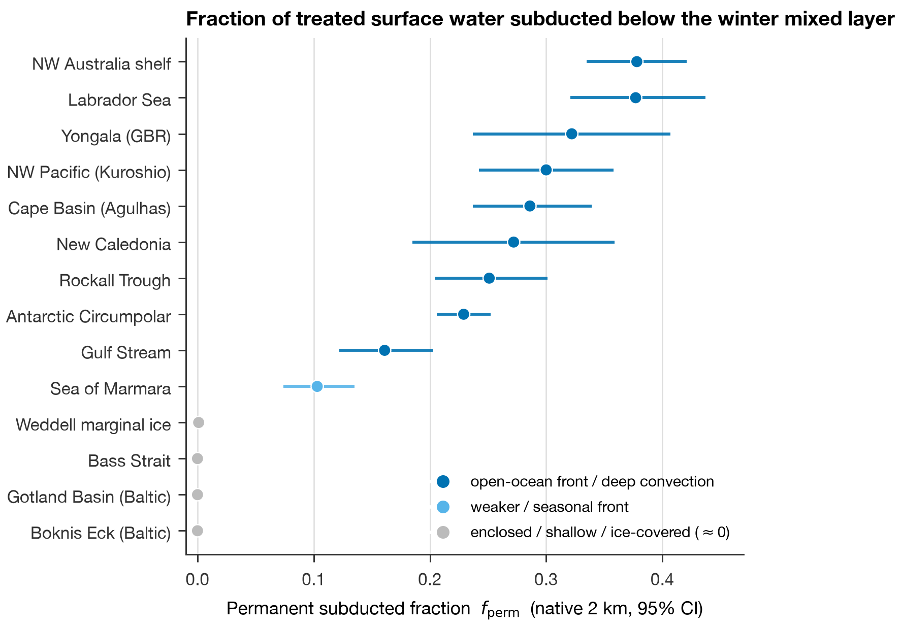
Table 1 and Fig. 2 give f100 at native resolution. In nine of the 14 subdomains between 0.16 and 0.38 of surviving particles sit below 100 m through the last quarter of a 16-day winter window: Labrador Sea 0.38, NW Australia 0.38, Yongala (Great Barrier Reef shelf) 0.32, NW Pacific 0.30, Agulhas (Cape Basin) 0.29, New Caledonia 0.27, Rockall Trough 0.25, ACC 0.23 and Gulf Stream 0.16 and 0.20 in January and February. The Marmara Sea gives 0.10. The Baltic (two boxes), Bass Strait and the Weddell marginal ice zone give 0.00 to 0.001. The high values are not confined to the classic open-ocean fronts. Three of the nine are tropical or subtropical shelf-edge subdomains off Australia and New Caledonia with winter mixed layers of 22 to 60 m in the reanalysis, where a 100 m crossing is unlikely to represent the winter mixed-layer base. The Gulf Stream value repeats across two months (0.16, 0.20). The naive intervals in Table 1 understate the uncertainty for the reasons in Sect. 2.4, and the ordering among the nine is not established.
3.2 The same fields filtered to 25 to 100 km
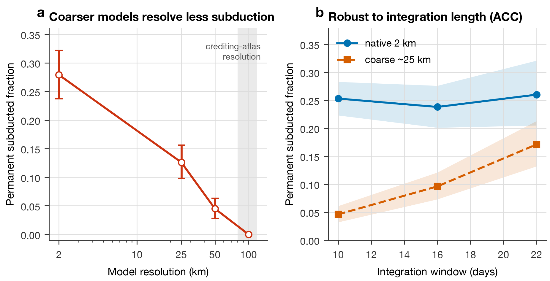
In the 16-day campaign the field filtered to 25 km gives f100 of 0.00 to 0.08 in every subdomain (largest: NW Australia 0.076, NW Pacific 0.059, Rockall Trough 0.030, Labrador Sea 0.019). The ACC July series, an 18-day window with 12-hourly snapshots and one seed set, gives 0.28 at 2 km, 0.13 at 25 km, 0.045 at 50 km and 0.00 at 100 km (Fig. 3a). The 25 km value in that series is larger than any 25 km value in the 16-day campaign, including the ACC August run (0.003), which used the same subdomain, a 16-day window and 6-hourly snapshots. The filtered-field fraction at 25 km is therefore not a stable number across months and windows. What is consistent is that it is a small fraction of the native value over these windows, and that at 100 km it is zero over 18 days.
Gross vertical exchange at the Gulf Stream tells a related story. The root-mean-square w on the boundary-layer base is 81 plus or minus 6 m per day at 2 km and 27 plus or minus 3 m per day at 25 km (ratio 2.97, bootstrap 95 percent interval over days 2.89 to 3.04), and the gross one-way downward flux is 24.9 versus 9.4 m per day (ratio 2.67, 2.51 to 2.79). Both quantities include reversible motion and neither is a transport across a moving boundary. The eNATL60 Mediterranean check gives ratios of 2.5 (w) and 2.0 (flux). These numbers say only that the filtered field has lost most of its vertical variance at the boundary-layer base.
3.3 Window dependence: the filtered field partially catches up
In the ACC July window series the native f100 stays near 0.25 (0.25, 0.24, 0.26 at 10, 16 and 22 days), while the 25 km fraction rises from 0.046 to 0.096 to 0.171 (Fig. 3b). The native-to-filtered ratio therefore falls from 5.5 to 2.5 to 1.5. Two things limit this series. Survivors fall from 810 to 467 to 215 particles (attrition 66, 80 and 91 percent), so the 22-day point rests on 215 survivors of 2374 seeded. And the series stops at 22 days, an order of magnitude short of tau_eq. Balwada et al. (2018) report about a 1.5 fold enhancement of tracer subduction between 1 and 20 km in an idealized channel. Our 22-day ratio matches that number, but the match is at one duration in a monotonically falling series and is not a validation. The question the series poses and does not answer is whether the 100 km field also catches up over the equilibration timescale. If it does, the effect on realized OAE uptake is a delay of weeks. If it does not, it is a horizon shift. [Pending rerun: native and 100 km f relative to the moving mixed-layer base over 180 days.]
3.4 Two models at the same front
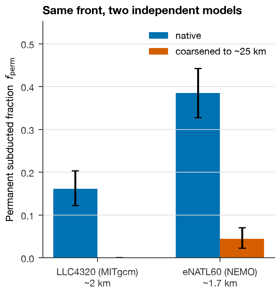
At the Gulf Stream, eNATL60 gives f100 = 0.39 (naive interval 0.33 to 0.44) at native resolution and 0.044 (0.022 to 0.070) at 25 km, from 278 survivors of 955 seeded (attrition 71 percent) over 17 days in February 2010 (Fig. 4). LLC4320 gives 0.16 and 0.20 in January and February 2012, pooled 0.18. The two models agree that a material fraction of surviving surface particles crosses 100 m within about two weeks and that the filtered field resolves much less of it. They disagree on the magnitude by a factor of 2.1 (extreme spread 1.6 to 2.8 using interval ends against the two months). The resolution difference between 1.7 and 2 km cannot produce that factor: extrapolating the ACC resolution series (Sect. 3.2) as the response curve. The remainder is attributable to model code, tides, the 2010 versus 2012 winter, the mixed-layer definition, the output cadence and the domain-exit censoring, in unknown proportion. We report the factor of two as structural uncertainty. Two configurations do not define a range for the effect, and we do not claim that either reproduces the other.
3.5 Coarse surface fields do not predict the crossing fraction
Across the six front and convection subdomains, a straight-line fit of f100 on the winter mixed-layer depth explains 4 percent of the variance, on front strength 18 percent, and on eddy kinetic energy 24 percent (Fig. S1). The H |grad b| proxy is anticorrelated with f100 across ten subdomains (r = -0.59), because the sharpest reanalysis gradients sit in the enclosed seas where f100 is near zero. At the one co-located pair, the Fox-Kemper velocity-scale estimate with its assumed net-to-gross ratio gives 0.24 for the Gulf Stream sites against a measured 0.16 to 0.20. These are six-point and ten-point fits on a hand-selected set with anti-conservative response intervals. They show that f100 is not predicted by the coarse surface fields we tested, with the fits we tried. They do not show that no parameterization exists, and they are not a test of the Fox-Kemper et al. (2008) closure as published.
3.6 Implementation sensitivities
The following are sensitivities of the implementation at the Gulf Stream (February 2012, native), not tests of the scientific inference. The instantaneous fraction of survivors below a reference depth at the end of the window is 0.46, 0.37 and 0.22 for 80, 100 and 150 m. The persistence-based f100 is 0.23, 0.20 and 0.17 for occupancy thresholds of 0.7, 0.8 and 0.9. Interpolating w on the model's w-faces rather than at cell centres gives 0.205 (522 survivors) against 0.199 (549). Adding an eddy diffusivity gives 0.223 (385 survivors), 12 percent above the base. A summer (August 2012) rerun in the Labrador Sea gives 0.27 (naive interval 0.16 to 0.39) from 56 survivors of 298 seeded, against 0.38 in February. That difference is inside the naive interval and is not evidence of seasonality. The August Gulf Stream box could not be seeded (14 columns met the seeding criterion and none survived). None of these variants addresses the fixed reference depth, the survivor-only denominator, the particle weighting or the non-conservative filtering, which are the dominant methodological limits.
4. Discussion
4.1 What the diagnostic does and does not establish
Within these experiments, a material fraction of surviving surface particles at open-ocean fronts, deep-convection sites and several shelf-edge subdomains crosses a 100 m reference depth within two to three weeks of a winter window and stays there through the end of it, and the same velocity fields filtered to 25 to 100 km resolve much less of that crossing over the same window. That is the result. It is a transport diagnostic in a model, on selected subdomains, in one winter, on survivors, at a fixed depth. It does not establish irreversible subduction, isolation from the atmosphere over months, or a return time. In the deep-convection subdomains the reference depth sits well inside the observed late-winter mixed layer (488 m in the Labrador Sea, 404 m in the subpolar northeast Atlantic), and in the shelf-edge subdomains it sits well below the reanalysis mixed layer, so f100 has a different physical meaning in different subdomains. The diagnostic that would resolve this is crossing relative to the local, time-varying mixed-layer base, followed long enough to record returns. That run is in progress.
4.2 Timescale comparison with air-sea equilibration
The crossing happens inside a 16 to 22-day window. The equilibration timescale we compute has a global median of 0.51 yr and site values of 0.17 to 0.72 yr, and Jones et al. (2014) give a similar range. The comparison is between two timescales, not a computed race. We have no crossing-time distribution to compare against a local, seasonally varying tau_eq, and we have not computed how much CO2 a parcel takes up before it crosses. The order-of-magnitude gap (weeks against months) is what motivates the coupled calculation. It is not itself an efficiency result.
4.3 Implication for OAE efficiency estimates
There is no identity between a crossing fraction and an efficiency loss. Realized uptake depends on the surface exposure history, dilution, buffer chemistry, gas transfer and later re-entrainment of the treated water, and the coarse efficiency models already contain their own resolved vertical transport, so an externally estimated fraction cannot be subtracted from them without double counting. What the present results support is qualitative: at frontal sites, part of the surface water an efficiency model treats as remaining in contact with the atmosphere over the first weeks has, in the submesoscale-resolving fields, left the surface layer by a route the filtered field does not carry. If that water re-ventilates on timescales longer than the crediting horizon, the model's near-term efficiency at such sites is too high, and the correction is a shift of realized uptake to a later horizon rather than a loss. The magnitude of that shift is not quantified here.
As an illustrative bound only, if a fraction f of the treated water at a site were removed before any uptake and did not return within the horizon, the near-term efficiency at that site would scale by (1 - f), with f in the 0.16 to 0.38 range of the frontal subdomains. That bound assumes the fixed-depth crossing is a permanent removal, which Sect. 4.1 explains is not established, and it ignores uptake before crossing. It is not a correction and should not be applied to any published atlas.
Re-ventilation timescales of the interior are known from the literature, not from these runs: years for mode waters that re-enter the winter mixed layer, and decades to centuries for water that reaches the permanent thermocline and below (Khatiwala et al., 2012). Our runs follow particles for at most 22 days and cannot say which of those fates the crossed particles meet. Zhou et al. (2024) attribute low modelled efficiency in some regions to subduction of the added alkalinity, so the mechanism is already part of the efficiency-model picture. What this paper adds is evidence that the submesoscale route is fast and is not carried by the filtered field.
4.4 Structural uncertainty and what the compute will add
The dominant uncertainties are structural and are not captured by the particle bootstrap: one winter, one year per model, two model configurations that disagree by a factor of two, a fixed reference depth, survivor-only denominators with 48 to 91 percent attrition, unweighted particles, and a non-conservative filter. The compute in progress addresses four of them: a moving mixed-layer base, 180-day windows that reach past tau_eq and record returns, per-particle records that allow column and spatial block bootstraps, and the full seed set with exited particles as a censored class. It does not address particle weighting, the filter, interannual variability or the coupled carbonate response. A passive alkalinity and DIC tracer run online in a submesoscale-resolving model with carbonate chemistry and gas exchange, in matched native and coarse configurations, remains the calculation that would turn this diagnostic into an efficiency statement.
4.5 Relation to prior work
Balwada et al. (2018) established the enhancement of passive-tracer subduction by submesoscale vertical velocities in an idealized channel. He and Tyka (2023) established that near-coast OAE realization depends on transport and equilibration. Zhou et al. (2024) and Tyka (2025) provide the efficiency models and the horizon dependence of their metric. Jones et al. (2014) provide the equilibration-timescale framework. Fox-Kemper et al. (2008) provide the mixed-layer-eddy closure. What is new here is narrow: a consistently defined crossing diagnostic in two realistic submesoscale-resolving simulations across 14 selected subdomains, its behaviour under spatial filtering to 25 to 100 km and under window length, and the placement of that diagnostic against the OAE equilibration timescale. The sign of any effect on other marine CDR methods depends on the species transported, its depth and its return time, and we do not generalize beyond dissolved alkalinity.
5. Conclusions
In two submesoscale-resolving models, 0.16 to 0.38 of surviving surface particles in nine of 14 selected subdomains cross a 100 m reference depth within a 16-day winter window and remain below it. The same velocity fields filtered to 25 km resolve 0.00 to 0.08 of that crossing at 16 days, 0.13 in an 18-day ACC series, and 0.00 at 100 km, and the 25 km fraction partially catches up between 10 and 22 days. The two models disagree by a factor of two at the Gulf Stream, the resolution difference alone cannot produce that gap, and the between-front ordering is not established under column clustering. The crossing takes weeks against an equilibration timescale of months. The OAE implication is a horizon shift at frontal sites of unquantified magnitude. A moving-mixed-layer, 180-day, block-bootstrap rerun is in progress, and a coupled carbonate calculation is the next step.
Code and data availability
Analysis code is in the private repository github.com/steps-re/marine-cdr-equilibration (branch research/submeso-corrected-viability), which will be made public at submission. Derived CSV outputs and figures are in the Google Cloud Storage bucket gs://airloom-marine-cdr/outputs (132 objects at the time of writing, access on request until the Zenodo record is minted). A Zenodo package with the derived CSVs, the publication figures and the analysis scripts is staged (outputs/zenodo_release) and no DOI has been reserved yet. Released: e_campaign_global.csv (Table 1), e_campaign.csv (both Gulf Stream months), coarsen_bracket.csv, acc_window_sweep.csv, enatl_gs_fperm.csv, enatl_check.csv, phase_e2_llc4320.csv, s1_predictors.csv, cross_validate.csv, phase_e1_eddy_subduction.csv, sensitivity_test.csv, offline_robust.csv, seasonal_test.csv, bgc_argo.csv. Not released: per-particle trajectory records (not retained for the runs reported here), the LLC4320 and eNATL60 subsets (deleted after each run to bound disk, and redistributable from source), and the GLORYS12 subsets. [Pending rerun: the rerun writes per-particle records (seed column, seed depth, final depth, persistence, native and filtered) that will be released with the Zenodo record.] Third-party sources: LLC4320 Pre-SWOT regional subsets from NASA PO.DAAC, eNATL60 from the SWOT-AdAC OSN archive (Pangeo/pangeo-forge/swot_adac/eNATL60/Region01/interior_daily/fma.zarr, endpoint https://ncsa.osn.xsede.org), GLORYS12 and wind stress from CMEMS, Argo via argopy.
Author contributions and competing interests
M. German designed the experiments, wrote the analysis code, ran the simulations and wrote the paper. Co-author slots are open and no other person has agreed to authorship. The author is the founder of Steps Ventures, which has no commercial interest in ocean alkalinity enhancement. No funding was received.
References
- Balwada, D., Smith, K. S., and Abernathey, R.: Submesoscale vertical velocities enhance tracer subduction in an idealized Antarctic Circumpolar Current, Geophys. Res. Lett., 45, 9790-9802, 2018.
- Brodeau, L., Le Sommer, J., and Albert, A.: Ocean-next/eNATL60: material describing the set-up and the assessment of NEMO-eNATL60 simulations, Zenodo, https://doi.org/10.5281/zenodo.4032732, 2020.
- Fox-Kemper, B., Ferrari, R., and Hallberg, R.: Parameterization of mixed layer eddies. Part I: Theory and diagnosis, J. Phys. Oceanogr., 38, 1145-1165, 2008.
- He, J. and Tyka, M. D.: Limits and CO2 equilibration of near-coast alkalinity enhancement, Biogeosciences, 20, 27-43, 2023.
- Humphreys, M. P., Lewis, E. R., Sharp, J. D., and Pierrot, D.: PyCO2SYS v1.8: marine carbonate system calculations in Python, Geosci. Model Dev., 15, 15-43, 2022.
- Jones, D. C., Ito, T., Takano, Y., and Hsu, W.-C.: Spatial and seasonal variability of the air-sea equilibration timescale of carbon dioxide, Global Biogeochem. Cy., 28, 1163-1178, 2014.
- Khatiwala, S., Primeau, F., and Holzer, M.: Ventilation of the deep ocean constrained with tracer observations and implications for radiocarbon estimates of ideal mean age, Earth Planet. Sc. Lett., 325-326, 116-125, 2012.
- Lévy, M., Ferrari, R., Franks, P. J. S., Martin, A. P., and Rivière, P.: Bringing physics to life at the submesoscale, Geophys. Res. Lett., 39, L14602, 2012.
- NASA JPL: Pre-SWOT Level-4 Hourly MITgcm LLC4320 Ocean Simulation Regional Subsets (MITgcm_LLC4320_Pre-SWOT_JPL_L4, version 1.0), NASA PO.DAAC, 2021.
- Omand, M. M., D'Asaro, E. A., Lee, C. M., Perry, M. J., Briggs, N., Cetinić, I., and Mahadevan, A.: Eddy-driven subduction exports particulate organic carbon from the spring bloom, Science, 348, 222-225, 2015.
- Su, Z., Wang, J., Klein, P., Thompson, A. F., and Menemenlis, D.: Ocean submesoscales as a key component of the global heat budget, Nat. Commun., 9, 775, 2018.
- Tyka, M. D.: Efficiency metrics for ocean alkalinity enhancement under responsive and prescribed atmospheric pCO2 conditions, Biogeosciences, 2025.
- Uchida, T., Le Sommer, J., Stern, C., et al.: Cloud-based framework for inter-comparing submesoscale-permitting realistic ocean models, Geosci. Model Dev., 15, 5829-5856, 2022.
- Wanninkhof, R.: Relationship between wind speed and gas exchange over the ocean revisited, Limnol. Oceanogr. Meth., 12, 351-362, 2014.
- Zhou, M., Tyka, M. D., Ho, D. T., Yankovsky, E., Bachman, S., Nicholas, T., Karspeck, A. R., and Long, M. C.: Mapping the global variation in the efficiency of ocean alkalinity enhancement for carbon dioxide removal, Nat. Clim. Change, 2024.
Table 1. Fraction f100 of surviving particles below the 100 m reference depth for at least 80 percent of the last quarter of a 16-day winter window, LLC4320, native (about 2 km) and the same field filtered to 25 km. Intervals are naive particle bootstraps (Sect. 2.4) and understate the uncertainty by at least a factor of the square root of three. An interval of [0.000, 0.000] means no crossing events among the survivors of that run. The bootstrap gives no upper bound in that case. Under independence the 95 percent upper bound is about 3 divided by the survivor count (0.01 for 311 survivors), and wider under clustering. Attrition is the fraction of seeded particles that left the subdomain or reached undefined velocity before the end of the window. Source: outputs/e_campaign_global.csv and outputs/e_campaign.csv. Reanalysis winter MLD is the GLORYS12 2019 winter maximum at the subdomain centre (outputs/s1_predictors.csv). [Pending rerun: replace with moving-mixed-layer f on the full seed set with block-bootstrap intervals.]
Table 1b. Rerun with per-particle output (paper/uq/block_bootstrap.py). f100 over survivors with the naive interval and the 50 km block-bootstrap interval, then the full-cohort crossed fraction with domain exit as a censored class, and the paired native-minus-25 km difference with its 25 km block interval.
| Region, month | f100 (survivors) | naive 95% | 50 km block 95% | full cohort crossed | censored | paired native minus 25 km |
|---|---|---|---|---|---|---|
| Gulf Stream, Jan 2012 | 0.161 | 0.122 to 0.203 | 0.091 to 0.242 | 0.045 | 0.72 | +0.14 (0.08 to 0.20) |
| Gulf Stream, Feb 2012 | 0.199 | 0.166 to 0.231 | 0.133 to 0.262 | 0.087 | 0.56 | +0.19 (0.15 to 0.24) |
| ACC, Jul 2012 | 0.236 | 0.196 to 0.278 | 0.174 to 0.306 | 0.039 | 0.83 | +0.18 (0.10 to 0.27) |
| ACC, Aug 2012 | 0.229 | 0.206 to 0.252 | 0.191 to 0.270 | 0.119 | 0.48 | +0.23 (0.20 to 0.26) |
| Subdomain | Setting | Month | Reanalysis winter MLD (m) | Seeded | Survived | Attrition | f100 native [naive 95%] | f100 filtered 25 km [naive 95%] |
|---|---|---|---|---|---|---|---|---|
| Labrador Sea | subpolar deep convection | Feb 2012 | 51 | 720 | 268 | 0.63 | 0.377 [0.321, 0.437] | 0.019 [0.009, 0.032] |
| NW Australia | tropical shelf edge | Jul 2012 | 56 | 735 | 484 | 0.34 | 0.378 [0.335, 0.421] | 0.076 [0.054, 0.099] |
| Yongala | Great Barrier Reef shelf | Jul 2012 | 22 | 224 | 118 | 0.47 | 0.322 [0.237, 0.407] | 0.010 [0.000, 0.024] |
| NW Pacific | subtropical counter-current, 20 N | Feb 2012 | 102 | 716 | 240 | 0.66 | 0.300 [0.242, 0.358] | 0.059 [0.035, 0.082] |
| Cape Basin | Agulhas retroflection | Jul 2012 | 150 | 859 | 304 | 0.65 | 0.286 [0.237, 0.339] | 0.000 [0.000, 0.000] |
| New Caledonia | subtropical, SW Pacific | Jul 2012 | 60 | 281 | 92 | 0.67 | 0.272 [0.185, 0.359] | 0.006 [0.000, 0.019] |
| Rockall Trough | subpolar NE Atlantic | Feb 2012 | 290 | 969 | 299 | 0.69 | 0.251 [0.204, 0.301] | 0.030 [0.019, 0.043] |
| ACC (SMST) | Antarctic Circumpolar Current | Aug 2012 | 171 | 2374 | 1236 | 0.48 | 0.229 [0.206, 0.252] | 0.003 [0.001, 0.007] |
| Gulf Stream (WestAtlantic) | western boundary current | Feb 2012 | 64 | 1257 | 549 | 0.56 | 0.199 [0.166, 0.231] | 0.007 [0.001, 0.014] |
| Gulf Stream (WestAtlantic) | western boundary current | Jan 2012 | 64 | 1103 | 311 | 0.72 | 0.161 [0.122, 0.203] | 0.000 [0.000, 0.000] |
| Marmara Sea | enclosed, strait-fed | Feb 2012 | 11 | 388 | 379 | 0.02 | 0.103 [0.074, 0.135] | 0.000 [0.000, 0.000] |
| Weddell MIZ (ROAM) | marginal ice zone | Aug 2012 | 116 | 689 | 677 | 0.02 | 0.001 [0.000, 0.004] | 0.000 [0.000, 0.000] |
| Bass Strait | shallow shelf strait | Jul 2012 | 72 | 480 | 415 | 0.14 | 0.000 [0.000, 0.000] | 0.000 [0.000, 0.000] |
| Gotland Basin | Baltic, enclosed | Feb 2012 | 46 | 1019 | 1019 | 0.00 | 0.000 [0.000, 0.000] | 0.000 [0.000, 0.000] |
| Boknis Eck | Baltic, enclosed | Feb 2012 | 11 | 339 | 321 | 0.05 | 0.000 [0.000, 0.000] | 0.000 [0.000, 0.000] |
Table 2. Cross-model and window-length runs. Same criterion as Table 1. Sources: outputs/enatl_gs_fperm.csv, outputs/coarsen_bracket.csv, outputs/acc_window_sweep.csv. The 100 km entry is zero events among an unrecorded number of survivors, not a measured zero, and the survivor counts for the resolution series were not written out.
| Run | Model | Window (d) | Seeded | Survived | f100 native [naive 95%] | f100 filtered [naive 95%] | Filter scale |
|---|---|---|---|---|---|---|---|
| Gulf Stream, Feb 2010 | eNATL60 | 17 | 955 | 278 | 0.385 [0.327, 0.442] | 0.044 [0.022, 0.070] | 25 km |
| ACC, Jul 2012, resolution series | LLC4320 | 18 | 2374 | n/a | 0.279 [0.237, 0.322] | 0.126 [0.098, 0.156] | 25 km |
| 0.045 [0.028, 0.063] | 50 km | ||||||
| 0.000 [0.000, 0.000] | 100 km | ||||||
| ACC, Jul 2012, window series | LLC4320 | 10 | 2374 | 810 | 0.253 [0.223, 0.283] | 0.046 [0.032, 0.061] | 25 km |
| 16 | 2374 | 467 | 0.238 [0.201, 0.276] | 0.096 [0.073, 0.121] | 25 km | ||
| 22 | 2374 | 215 | 0.260 [0.205, 0.321] | 0.171 [0.132, 0.213] | 25 km |
Figures
Figure files are in outputs/figs_ncc. Their current axis labels and titles still read "permanent subducted fraction" and "not parameterizable" and will be regenerated with the rerun. [Pending rerun: regenerate all figures with the moving-mixed-layer diagnostic and block-bootstrap intervals, and relabel.]
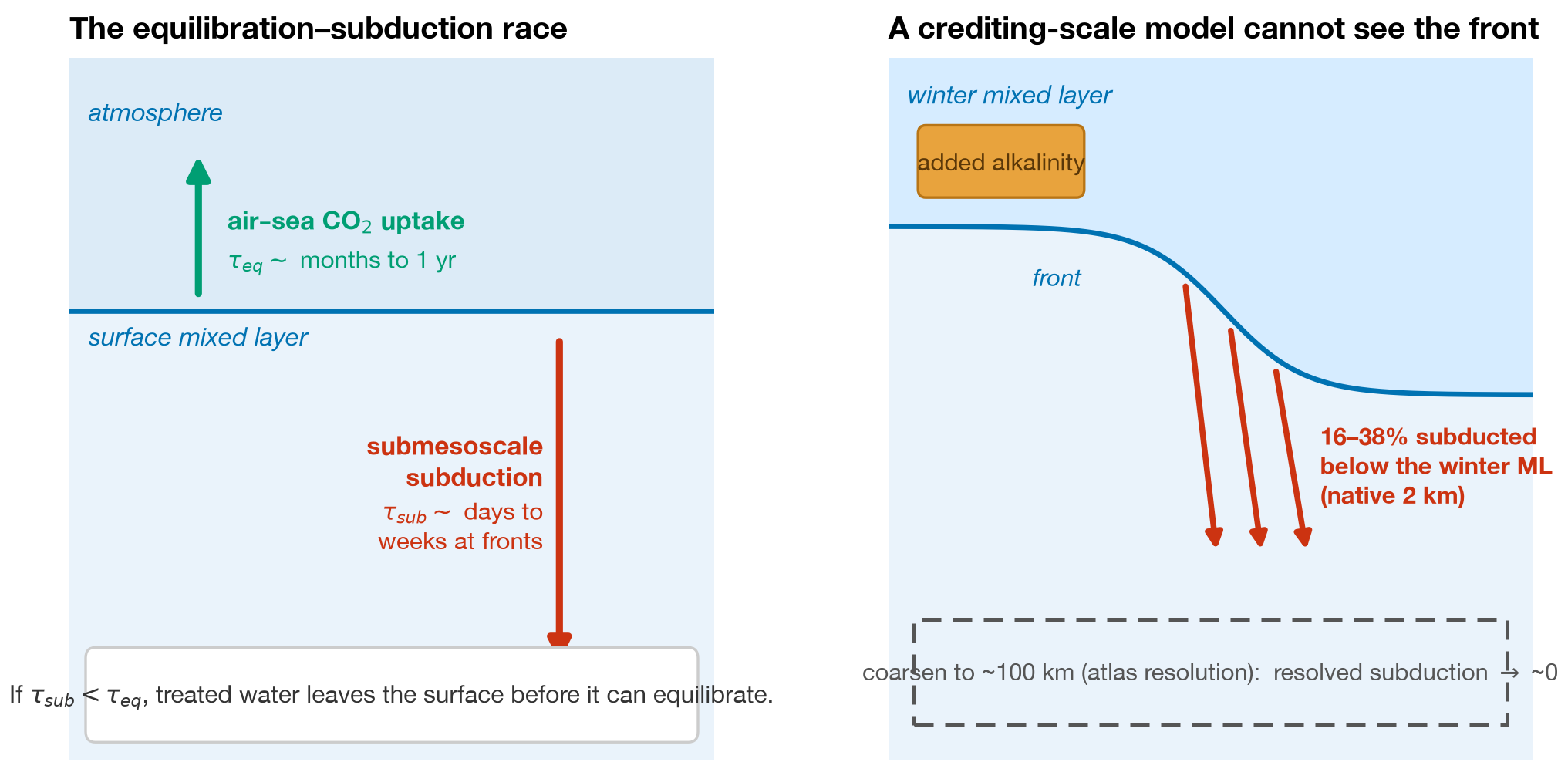
- Fig. 1. Schematic of the timescale comparison: horizontal dilution conserves the surface integral of an added tracer, vertical transport below the mixed-layer base defers its air-sea equilibration. (fig1_schematic)
- Fig. 2. f100 at native resolution across the 14 LLC4320 subdomains, ordered by magnitude, with naive particle-bootstrap intervals. Colours mark front and convection, shelf, and enclosed or ice-covered settings. (fig2_region_result. The error bars are the naive intervals of Sect. 2.4.)
- Fig. 3. (a) f100 in the ACC July 2012 series versus filter scale (2, 25, 50, 100 km). (b) Native and 25 km f100 versus window length (10, 16, 22 days) in the same subdomain and seed set, with survivor counts. (fig3_robustness)
- Fig. 4. The same Gulf Stream front in LLC4320 (January and February 2012) and eNATL60 (February 2010): native and 25 km f100. (fig4_cross_model)
- Fig. S1. f100 against reanalysis winter mixed-layer depth, surface buoyancy-gradient magnitude and eddy kinetic energy for the six fitted front and convection subdomains, with the eight hold-outs shown. (figS1_predictors)
- Fig. S2. Root-mean-square w and gross one-way downward flux on the boundary-layer base, native versus 25 km, in LLC4320 (Gulf Stream) and eNATL60 (Mediterranean subdomain). (figS2_cross_model_wexchange)